Electricity Transformer Temperature

概要

電力変圧器温度に関する多変量時系列データセット。中国の2つの地区で、2年間取得されている。いずれも目的変数の"oil temperature"と、ほかの6つの特徴量が含まれている。

• オリジナルデータ： GitHub

• データ形式: .csv

• タスク: 時系列予測

データスペック

データ長:

2年間

特徴量次元:

7 (うちoil temperature が目的変数)

サンプリング間隔:

ファイル名の1 と2 はデータ収集場所の違い

• ETTh1.csv, ETTh2.csv は1時間ごと

• ETTm1.csv, ETTm2.csv は15分ごと

バリデーション:

元論文（Informer）中では、Train/Vaild/Testを、それぞれ12/4/4ヵ月に分割して使用

カラム名

csvファイルに格納されているカラム名の略記一覧

Field	date	HUFL	HULL	MUFL	MULL	LUFL	LULL	OT
Description	The recorded date	High UseFul Load	High UseLess Load	Middle UseFul Load	Middle UseLess Load	Low UseFul Load	Low UseLess Load	Oil Temperature (target)

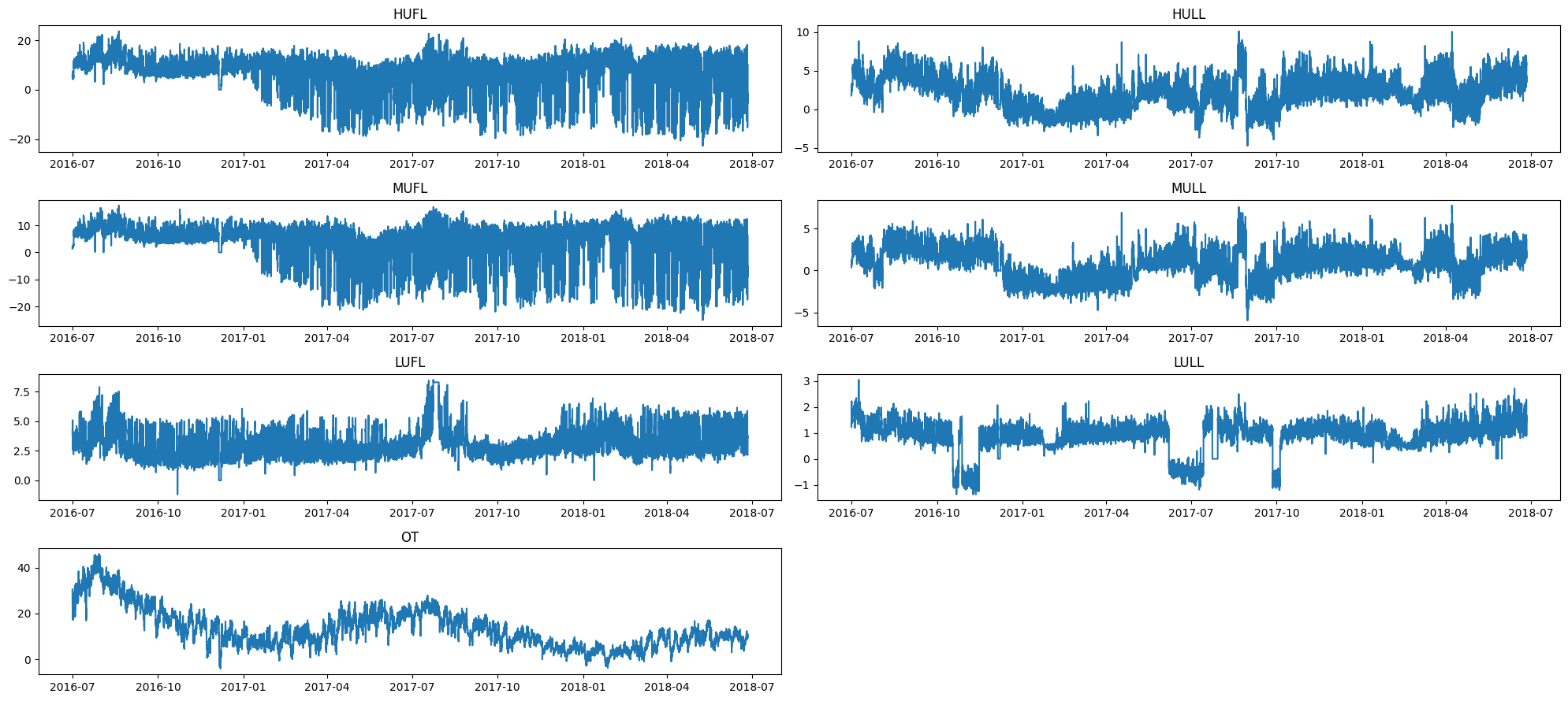
可視化

前述のGitHubリポジトリからデータをダウンロードしていることとします。

ここではcsvファイルを ../data/ETT-small に配置したと想定して可視化します。また、ETTh1のみを例示します。

ライブラリ群の読み込み （折りたたみ）

Show code cell source Hide code cell source

from pathlib import Path

import numpy as np
import matplotlib.pyplot as plt
import pandas as pd
import seaborn as sns
import plotly.graph_objects as go
from plotly.subplots import make_subplots
import plotly.io as pio
import plotly.express as px
import plotly.offline as py
from plotly_resampler import FigureResampler

pio.renderers.default = "plotly_mimetype+notebook"

データ読み込み

rootdir = Path("../data/ETT-small")

ETTh1 = pd.read_csv(rootdir / "ETTh1.csv", index_col=0, parse_dates=True)
ETTh2 = pd.read_csv(rootdir / "ETTh2.csv", index_col=0, parse_dates=True)
ETTm1 = pd.read_csv(rootdir / "ETTm1.csv", index_col=0, parse_dates=True)
ETTm2 = pd.read_csv(rootdir / "ETTm2.csv", index_col=0, parse_dates=True)

ETTh1.head()

	HUFL	HULL	MUFL	MULL	LUFL	LULL	OT
date
2016-07-01 00:00:00	5.827	2.009	1.599	0.462	4.203	1.340	30.531000
2016-07-01 01:00:00	5.693	2.076	1.492	0.426	4.142	1.371	27.787001
2016-07-01 02:00:00	5.157	1.741	1.279	0.355	3.777	1.218	27.787001
2016-07-01 03:00:00	5.090	1.942	1.279	0.391	3.807	1.279	25.044001
2016-07-01 04:00:00	5.358	1.942	1.492	0.462	3.868	1.279	21.948000

ETTh1.describe()

	HUFL	HULL	MUFL	MULL	LUFL	LULL	OT
count	17420.000000	17420.000000	17420.000000	17420.000000	17420.000000	17420.000000	17420.000000
mean	7.375141	2.242242	4.300239	0.881568	3.066062	0.856932	13.324672
std	7.067744	2.042342	6.826978	1.809293	1.164506	0.599552	8.566946
min	-22.705999	-4.756000	-25.087999	-5.934000	-1.188000	-1.371000	-4.080000
25%	5.827000	0.737000	3.296000	-0.284000	2.315000	0.670000	6.964000
50%	8.774000	2.210000	5.970000	0.959000	2.833000	0.975000	11.396000
75%	11.788000	3.684000	8.635000	2.203000	3.625000	1.218000	18.079000
max	23.643999	10.114000	17.341000	7.747000	8.498000	3.046000	46.007000

プロット (Plotly)

fig = make_subplots(
    rows=7, shared_xaxes=True, vertical_spacing=0.04, subplot_titles=ETTh1.columns
)
fig = FigureResampler(fig)

idx = ETTh1.index
for i, col in enumerate(ETTh1.columns):
    fig.add_trace(go.Scattergl(x=idx, y=ETTh1[col], name=col), row=i + 1, col=1)
fig.update_layout(
    autosize=True, height=1000, margin=dict(l=20, r=20, t=20, b=10), showlegend=False
)
fig.show()

補足: matplotlibの場合

Show code cell content Hide code cell content

import math


def plot_ts(df: pd.DataFrame, n_split=2, dpi=100):
    n_col = len(df.columns)
    fig = plt.figure(figsize=(20, n_col // n_split * 3), dpi=dpi)
    x_idx = df.index

    for i, c in enumerate(df.columns):
        ax = fig.add_subplot(math.ceil(n_col / n_split), n_split, i + 1)
        ax.set_title(c)
        ax.plot(x_idx, df[c])

    plt.tight_layout()
    plt.show()


plot_ts(ETTh1)

参考文献

• Zhou, Haoyi, et al. "Informer: Beyond efficient transformer for long sequence time-series forecasting." Proceedings of the AAAI Conference on Artificial Intelligence. Vol. 35. No. 12. 2021.